Bloch-Redfield master equation

Introduction

The Lindblad master equation introduced earlier is constructed so that it describes a physical evolution of the density matrix (i.e., trace and positivity preserving), but it does not provide a connection to any underlying microscopic physical model. The Lindblad operators (collapse operators) describe phenomenological processes, such as for example dephasing and spin flips, and the rates of these processes are arbitrary parameters in the model. In many situations the collapse operators and their corresponding rates have clear physical interpretation, such as dephasing and relaxation rates, and in those cases the Lindblad master equation is usually the method of choice.

However, in some cases, for example systems with varying energy biases and eigenstates and that couple to an environment in some well-defined manner (through a physically motivated system-environment interaction operator), it is often desirable to derive the master equation from more fundamental physical principles, and relate it to for example the noise-power spectrum of the environment.

The Bloch-Redfield formalism is one such approach to derive a master equation from a microscopic system. It starts from a combined system-environment perspective, and derives a perturbative master equation for the system alone, under the assumption of weak system-environment coupling. One advantage of this approach is that the dissipation processes and rates are obtained directly from the properties of the environment. On the downside, it does not intrinsically guarantee that the resulting master equation unconditionally preserves the physical properties of the density matrix (because it is a perturbative method). The Bloch-Redfield master equation must therefore be used with care, and the assumptions made in the derivation must be honored. (The Lindblad master equation is in a sense more robust – it always results in a physical density matrix – although some collapse operators might not be physically justified). For a full derivation of the Bloch Redfield master equation, see e.g. [Coh92] or [Bre02]. Here we present only a brief version of the derivation, with the intention of introducing the notation and how it relates to the implementation in QuTiP.

Brief Derivation and Definitions

The starting point of the Bloch-Redfield formalism is the total Hamiltonian for the system and the environment (bath): \(H = H_{\rm S} + H_{\rm B} + H_{\rm I}\), where \(H\) is the total system+bath Hamiltonian, \(H_{\rm S}\) and \(H_{\rm B}\) are the system and bath Hamiltonians, respectively, and \(H_{\rm I}\) is the interaction Hamiltonian.

The most general form of a master equation for the system dynamics is obtained by tracing out the bath from the von-Neumann equation of motion for the combined system (\(\dot\rho = -i\hbar^{-1}[H, \rho]\)). In the interaction picture the result is

(1)\[ \frac{d}{dt}\rho_S(t) = - \hbar^{-2}\int_0^t d\tau\; {\rm Tr}_B [H_I(t), [H_I(\tau), \rho_S(\tau)\otimes\rho_B]],\]

where the additional assumption that the total system-bath density matrix can be factorized as \(\rho(t) \approx \rho_S(t) \otimes \rho_B\). This assumption is known as the Born approximation, and it implies that there never is any entanglement between the system and the bath, neither in the initial state nor at any time during the evolution. It is justified for weak system-bath interaction.

The master equation (1) is non-Markovian, i.e., the change in the density matrix at a time \(t\) depends on states at all times \(\tau < t\), making it intractable to solve both theoretically and numerically. To make progress towards a manageable master equation, we now introduce the Markovian approximation, in which \(\rho_S(\tau)\) is replaced by \(\rho_S(t)\) in Eq. (1). The result is the Redfield equation

(2)\[ \frac{d}{dt}\rho_S(t) = - \hbar^{-2}\int_0^t d\tau\; {\rm Tr}_B [H_I(t), [H_I(\tau), \rho_S(t)\otimes\rho_B]],\]

which is local in time with respect the density matrix, but still not Markovian since it contains an implicit dependence on the initial state. By extending the integration to infinity and substituting \(\tau \rightarrow t-\tau\), a fully Markovian master equation is obtained:

(3)\[ \frac{d}{dt}\rho_S(t) = - \hbar^{-2}\int_0^\infty d\tau\; {\rm Tr}_B [H_I(t), [H_I(t-\tau), \rho_S(t)\otimes\rho_B]].\]

The two Markovian approximations introduced above are valid if the time-scale with which the system dynamics changes is large compared to the time-scale with which correlations in the bath decays (corresponding to a “short-memory” bath, which results in Markovian system dynamics).

The master equation (3) is still on a too general form to be suitable for numerical implementation. We therefore assume that the system-bath interaction takes the form \(H_I = \sum_\alpha A_\alpha \otimes B_\alpha\) and where \(A_\alpha\) are system operators and \(B_\alpha\) are bath operators. This allows us to write master equation in terms of system operators and bath correlation functions:

\[\begin{split}\frac{d}{dt}\rho_S(t) = -\hbar^{-2} \sum_{\alpha\beta} \int_0^\infty d\tau\; \left\{ g_{\alpha\beta}(\tau) \left[A_\alpha(t)A_\beta(t-\tau)\rho_S(t) - A_\alpha(t-\tau)\rho_S(t)A_\beta(t)\right] \right. \nonumber\\ \left. g_{\alpha\beta}(-\tau) \left[\rho_S(t)A_\alpha(t-\tau)A_\beta(t) - A_\alpha(t)\rho_S(t)A_\beta(t-\tau)\right] \right\},\end{split}\]

where \(g_{\alpha\beta}(\tau) = {\rm Tr}_B\left[B_\alpha(t)B_\beta(t-\tau)\rho_B\right] = \left<B_\alpha(\tau)B_\beta(0)\right>\), since the bath state \(\rho_B\) is a steady state.

In the eigenbasis of the system Hamiltonian, where \(A_{mn}(t) = A_{mn} e^{i\omega_{mn}t}\), \(\omega_{mn} = \omega_m - \omega_n\) and \(\omega_m\) are the eigenfrequencies corresponding the eigenstate \(\left|m\right>\), we obtain in matrix form in the Schrödinger picture

\[\begin{split}\frac{d}{dt}\rho_{ab}(t) =& -i\omega_{ab}\rho_{ab}(t) \nonumber\\ &-\hbar^{-2} \sum_{\alpha,\beta} \sum_{c,d}^{\rm sec} \int_0^\infty d\tau\; \left\{ g_{\alpha\beta}(\tau) \left[\delta_{bd}\sum_nA^\alpha_{an}A^\beta_{nc}e^{i\omega_{cn}\tau} - A^\alpha_{ac} A^\beta_{db} e^{i\omega_{ca}\tau} \right] \right. \nonumber\\ &+ \left. g_{\alpha\beta}(-\tau) \left[\delta_{ac}\sum_n A^\alpha_{dn}A^\beta_{nb} e^{i\omega_{nd}\tau} - A^\alpha_{ac}A^\beta_{db}e^{i\omega_{bd}\tau} \right] \right\} \rho_{cd}(t), \nonumber\\\end{split}\]

where the “sec” above the summation symbol indicate summation of the secular terms which satisfy \(|\omega_{ab}-\omega_{cd}| \ll \tau_ {\rm decay}\). This is an almost-useful form of the master equation. The final step before arriving at the form of the Bloch-Redfield master equation that is implemented in QuTiP, involves rewriting the bath correlation function \(g(\tau)\) in terms of the noise-power spectrum of the environment \(S(\omega) = \int_{-\infty}^\infty d\tau e^{i\omega\tau} g(\tau)\):

(4)\[ \int_0^\infty d\tau\; g_{\alpha\beta}(\tau) e^{i\omega\tau} = \frac{1}{2}S_{\alpha\beta}(\omega) + i\lambda_{\alpha\beta}(\omega),\]

where \(\lambda_{ab}(\omega)\) is an energy shift that is neglected here. The final form of the Bloch-Redfield master equation is

(5)\[\frac{d}{dt}\rho_{ab}(t) = -i\omega_{ab}\rho_{ab}(t) + \sum_{c,d}^{\rm sec}R_{abcd}\rho_{cd}(t),\]

where

(6)\[\begin{split} R_{abcd} = -\frac{\hbar^{-2}}{2} \sum_{\alpha,\beta} \left\{ \delta_{bd}\sum_nA^\alpha_{an}A^\beta_{nc}S_{\alpha\beta}(\omega_{cn}) - A^\alpha_{ac} A^\beta_{db} S_{\alpha\beta}(\omega_{ca}) \right. \nonumber\\ + \left. \delta_{ac}\sum_n A^\alpha_{dn}A^\beta_{nb} S_{\alpha\beta}(\omega_{dn}) - A^\alpha_{ac}A^\beta_{db} S_{\alpha\beta}(\omega_{db}) \right\},\end{split}\]

is the Bloch-Redfield tensor.

The Bloch-Redfield master equation in the form Eq. (5) is suitable for numerical implementation. The input parameters are the system Hamiltonian \(H\), the system operators through which the environment couples to the system \(A_\alpha\), and the noise-power spectrum \(S_{\alpha\beta}(\omega)\) associated with each system-environment interaction term.

To simplify the numerical implementation we assume that \(A_\alpha\) are Hermitian and that cross-correlations between different environment operators vanish, so that the final expression for the Bloch-Redfield tensor that is implemented in QuTiP is

(7)\[\begin{split} R_{abcd} = -\frac{\hbar^{-2}}{2} \sum_{\alpha} \left\{ \delta_{bd}\sum_nA^\alpha_{an}A^\alpha_{nc}S_{\alpha}(\omega_{cn}) - A^\alpha_{ac} A^\alpha_{db} S_{\alpha}(\omega_{ca}) \right. \nonumber\\ + \left. \delta_{ac}\sum_n A^\alpha_{dn}A^\alpha_{nb} S_{\alpha}(\omega_{dn}) - A^\alpha_{ac}A^\alpha_{db} S_{\alpha}(\omega_{db}) \right\}.\end{split}\]

Bloch-Redfield master equation in QuTiP

In QuTiP, the Bloch-Redfield tensor Eq. (7) can be calculated using the function bloch_redfield_tensor. It takes two mandatory arguments: The system Hamiltonian \(H\), a nested list of operator \(A_\alpha\), spectral density functions \(S_\alpha(\omega)\) pairs that characterize the coupling between system and bath. The spectral density functions are Python callback functions that takes the (angular) frequency as a single argument.

To illustrate how to calculate the Bloch-Redfield tensor, let’s consider a two-level atom

(8)\[ H = -\frac{1}{2}\Delta\sigma_x - \frac{1}{2}\epsilon_0\sigma_z\]

delta = 0.2 * 2*np.pi
eps0 = 1.0 * 2*np.pi
gamma1 = 0.5

H = - delta/2.0 * sigmax() - eps0/2.0 * sigmaz()

def ohmic_spectrum(w):
  if w == 0.0: # dephasing inducing noise
    return gamma1
  else: # relaxation inducing noise
    return gamma1 / 2 * (w / (2 * np.pi)) * (w > 0.0)


R, ekets = bloch_redfield_tensor(H, a_ops=[[sigmax(), ohmic_spectrum]])

print(R)

Output:

Quantum object: dims = [[[2], [2]], [[2], [2]]], shape = (4, 4), type = super, isherm = False
Qobj data =
[[ 0.        +0.j         0.        +0.j         0.        +0.j
   0.24514517+0.j       ]
 [ 0.        +0.j        -0.16103412-6.4076169j  0.        +0.j
   0.        +0.j       ]
 [ 0.        +0.j         0.        +0.j        -0.16103412+6.4076169j
   0.        +0.j       ]
 [ 0.        +0.j         0.        +0.j         0.        +0.j
  -0.24514517+0.j       ]]

Note that it is also possible to add Lindblad dissipation superoperators in the Bloch-Refield tensor by passing the operators via the c_ops keyword argument like you would in the mesolve or mcsolve functions. For convenience, the function bloch_redfield_tensor also returns the basis transformation operator, the eigen vector matrix, since they are calculated in the process of calculating the Bloch-Redfield tensor R, and the ekets are usually needed again later when transforming operators between the laboratory basis and the eigen basis. The tensor can be obtained in the laboratory basis by setting fock_basis=True, in that case, the transformation operator is not returned.

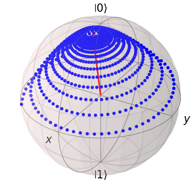
The evolution of a wavefunction or density matrix, according to the Bloch-Redfield master equation (5), can be calculated using the QuTiP function mesolve using Bloch-Refield tensor in the laboratory basis instead of a liouvillian. For example, to evaluate the expectation values of the \(\sigma_x\), \(\sigma_y\), and \(\sigma_z\) operators for the example above, we can use the following code:

delta = 0.2 * 2*np.pi
eps0 = 1.0 * 2*np.pi
gamma1 = 0.5

H = - delta/2.0 * sigmax() - eps0/2.0 * sigmaz()

def ohmic_spectrum(w):
    if w == 0.0: # dephasing inducing noise
        return gamma1
    else: # relaxation inducing noise
        return gamma1 / 2 * (w / (2 * np.pi)) * (w > 0.0)

R = bloch_redfield_tensor(H, [[sigmax(), ohmic_spectrum]], fock_basis=True)

tlist = np.linspace(0, 15.0, 1000)

psi0 = rand_ket(2, seed=1)

e_ops = [sigmax(), sigmay(), sigmaz()]

expt_list = mesolve(R, psi0, tlist, e_ops=e_ops).expect

sphere = Bloch()

sphere.add_points([expt_list[0], expt_list[1], expt_list[2]])

sphere.vector_color = ['r']

sphere.add_vectors(np.array([delta, 0, eps0]) / np.sqrt(delta ** 2 + eps0 ** 2))

sphere.make_sphere()

../../_images/dynamics-bloch-redfield-2.png

The two steps of calculating the Bloch-Redfield tensor and evolving according to the corresponding master equation can be combined into one by using the function brmesolve, which takes same arguments as mesolve and mcsolve, save for the additional nested list of operator-spectrum pairs that is called a_ops.

output = brmesolve(H, psi0, tlist, a_ops=[[sigmax(),ohmic_spectrum]], e_ops=e_ops)

where the resulting output is an instance of the class Result.

Note

While the code example simulates the Bloch-Redfield equation in the secular approximation, QuTiP’s implementation allows the user to simulate the non-secular version of the Bloch-Redfield equation by setting sec_cutoff=-1, as well as do a partial secular approximation by setting it to a float , this float will become the cutoff for the sum in (5) meaning terms with \(|\omega_{ab}-\omega_{cd}|\) greater than the cutoff will be neglected. Its default value is 0.1 which corresponds to the secular approximation. For example the command

output = brmesolve(H, psi0, tlist, a_ops=[[sigmax(), ohmic_spectrum]],
                   e_ops=e_ops, sec_cutoff=-1)

will simulate the same example as above without the secular approximation. Note that using the non-secular version may lead to negativity issues.

Time-dependent Bloch-Redfield Dynamics

If you have not done so already, please read the section: Solving Problems with Time-dependent Hamiltonians.

As we have already discussed, the Bloch-Redfield master equation requires transforming into the eigenbasis of the system Hamiltonian. For time-independent systems, this transformation need only be done once. However, for time-dependent systems, one must move to the instantaneous eigenbasis at each time-step in the evolution, thus greatly increasing the computational complexity of the dynamics. In addition, the requirement for computing all the eigenvalues severely limits the scalability of the method. Fortunately, this eigen decomposition occurs at the Hamiltonian level, as opposed to the super-operator level, and thus, with efficient programming, one can tackle many systems that are commonly encountered.

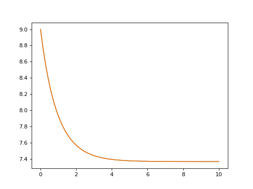
For time-dependent Hamiltonians, the Hamiltonian itself can be passed into the solver like any other time dependent Hamiltonian, as thus we will not discuss this topic further. Instead, here the focus is on time-dependent bath coupling terms. To this end, suppose that we have a dissipative harmonic oscillator, where the white-noise dissipation rate decreases exponentially with time \(\kappa(t) = \kappa(0)\exp(-t)\). In the Lindblad or Monte Carlo solvers, this could be implemented as a time-dependent collapse operator list c_ops = [[a, 'sqrt(kappa*exp(-t))']]. In the Bloch-Redfield solver, the bath coupling terms must be Hermitian. As such, in this example, our coupling operator is the position operator a+a.dag(). The complete example, and comparison to the analytic expression is:

N = 10  # number of basis states to consider
a = destroy(N)
H = a.dag() * a
psi0 = basis(N, 9)  # initial state
kappa = 0.2  # coupling to oscillator
a_ops = [
    ([a+a.dag(), f'sqrt({kappa}*exp(-t))'], '(w>=0)')
]
tlist = np.linspace(0, 10, 100)

out = brmesolve(H, psi0, tlist, a_ops, e_ops=[a.dag() * a])
actual_answer = 9.0 * np.exp(-kappa * (1.0 - np.exp(-tlist)))

plt.figure()
plt.plot(tlist, out.expect[0])
plt.plot(tlist, actual_answer)
plt.show()

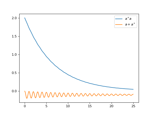
../../_images/dynamics-bloch-redfield-4.png

In many cases, the bath-coupling operators can take the form \(A = f(t)a + f(t)^* a^{+}\). The operator parts of the a_ops can be made of as many time-dependent terms as needed to construct such operator. For example consider a white-noise bath that is coupled to an operator of the form exp(1j*t)*a + exp(-1j*t)* a.dag(). In this example, the a_ops list would be:

a_ops = [
    ([[a, 'exp(1j*t)'], [a.dag(), 'exp(-1j*t)']], f'{kappa} * (w >= 0)')
]

where the first tuple element [[a, 'exp(1j*t)'], [a.dag(), 'exp(-1j*t)']] tells the solver what is the time-dependent Hermitian coupling operator. The second tuple f'{kappa} * (w >= 0)', gives the noise power spectrum. A full example is:

N = 10
w0 = 1.0 * 2 * np.pi
g = 0.05 * w0
kappa = 0.15
times = np.linspace(0, 25, 1000)

a = destroy(N)
H = w0 * a.dag() * a + g * (a + a.dag())
psi0 = ket2dm((basis(N, 4) + basis(N, 2) + basis(N, 0)).unit())
a_ops = [[
    QobjEvo([[a, 'exp(1j*t)'], [a.dag(), 'exp(-1j*t)']]), (f'{kappa} * (w >= 0)')
]]
e_ops = [a.dag() * a, a + a.dag()]

res_brme = brmesolve(H, psi0, times, a_ops, e_ops)

plt.figure()
plt.plot(times, res_brme.expect[0], label=r'$a^{+}a$')
plt.plot(times, res_brme.expect[1], label=r'$a+a^{+}$')
plt.legend()
plt.show()

../../_images/dynamics-bloch-redfield-6.png

Further examples on time-dependent Bloch-Redfield simulations can be found in the online tutorials.