Solving for Steady-State Solutions

Introduction

For time-independent open quantum systems with decay rates larger than the corresponding excitation rates, the system will tend toward a steady state as \(t\rightarrow\infty\) that satisfies the equation

\[\frac{d\hat{\rho}_{ss}}{dt}=\mathcal{L}\hat{\rho}_{ss}=0.\]

Although the requirement for time-independence seems quite resitrictive, one can often employ a transformation to the interaction picture that yields a time-independent Hamiltonian. For many these systems, solving for the asymptotic density matrix \(\hat{\rho}_{ss}\) can be achieved using direct or iterative solution methods faster than using master equation or Monte Carlo simulations. Although the steady state equation has a simple mathematical form, the properties of the Liouvillian operator are such that the solutions to this equation are anything but straightforward to find.

Steady State solvers in QuTiP

In QuTiP, the steady-state solution for a system Hamiltonian or Liouvillian is given by steadystate. This function implements a number of different methods for finding the steady state, each with their own pros and cons, where the method used can be chosen using the method keyword argument.

Method	Keyword	Description
Direct (default)	‘direct’	Direct solution solving \(Ax=b\).
Eigenvalue	‘eigen’	Iteratively find the zero eigenvalue of \(\mathcal{L}\).
Inverse-Power	‘power’	Solve using the inverse-power method.
SVD	‘svd’	Steady-state solution via the dense SVD of the Liouvillian.

The function steadystate can take either a Hamiltonian and a list of collapse operators as input, generating internally the corresponding Liouvillian super operator in Lindblad form, or alternatively, a Liouvillian passed by the user.

Both the "direct" and "power" method need to solve a linear equation system. To do so, there are multiple solvers available: ``

Solver	Original function	Description
“solve”	`numpy.linalg.solve`	Dense solver from numpy.
“lstsq”	`numpy.linalg.lstsq`	Dense least-squares solver.
“spsolve”	`scipy.sparse.linalg.spsolve`	Sparse solver from scipy.
“gmres”	`scipy.sparse.linalg.gmres`	Generalized Minimal RESidual iterative solver.
“lgmres”	`scipy.sparse.linalg.lgmres`	LGMRES iterative solver.
“bicgstab”	`scipy.sparse.linalg.bicgstab`	BIConjugate Gradient STABilized iterative solver.
“mkl_spsolve”	`pardiso`	Intel Pardiso LU solver from MKL

QuTiP can take advantage of the Intel Pardiso LU solver in the Intel Math Kernel library that comes with the Anacoda (2.5+) and Intel Python distributions. This gives a substantial increase in performance compared with the standard SuperLU method used by SciPy. To verify that QuTiP can find the necessary libraries, one can check for INTEL MKL Ext: True in the QuTiP about box (about).

Using the Steadystate Solver

Solving for the steady state solution to the Lindblad master equation for a general system with steadystate can be accomplished using:

>>> rho_ss = steadystate(H, c_ops)

where H is a quantum object representing the system Hamiltonian, and c_ops is a list of quantum objects for the system collapse operators. The output, labelled as rho_ss, is the steady-state solution for the systems. If no other keywords are passed to the solver, the default ‘direct’ method is used with numpy.linalg.solve, generating a solution that is exact to machine precision at the expense of a large memory requirement. However Liouvillians are often quite sparse and using a sparse solver may be preferred:

rho_ss = steadystate(H, c_ops, method="power", solver="spsolve")

where method='power' indicates that we are using the inverse-power solution method, and solver="spsolve" indicate to use the sparse solver.

Sparse solvers may still use quite a large amount of memory when they factorize the matrix since the Liouvillian usually has a large bandwidth. To address this, steadystate allows one to use the bandwidth minimization algorithms listed in Additional Solver Arguments. For example:

rho_ss = steadystate(H, c_ops, solver="spsolve", use_rcm=True)

where use_rcm=True turns on a bandwidth minimization routine.

Although it is not obvious, the 'direct', 'eigen', and 'power' methods all use an LU decomposition internally and thus can have a large memory overhead. In contrast, iterative solvers such as the 'gmres', 'lgmres', and 'bicgstab' do not factor the matrix and thus take less memory than the LU methods and allow, in principle, for extremely large system sizes. The downside is that these methods can take much longer than the direct method as the condition number of the Liouvillian matrix is large, indicating that these iterative methods require a large number of iterations for convergence. To overcome this, one can use a preconditioner \(M\) that solves for an approximate inverse for the (modified) Liouvillian, thus better conditioning the problem, leading to faster convergence. The use of a preconditioner can actually make these iterative methods faster than the other solution methods. The problem with precondioning is that it is only well defined for Hermitian matrices. Since the Liouvillian is non-Hermitian, the ability to find a good preconditioner is not guaranteed. And moreover, if a preconditioner is found, it is not guaranteed to have a good condition number. QuTiP can make use of an incomplete LU preconditioner when using the iterative 'gmres', 'lgmres', and 'bicgstab' solvers by setting use_precond=True. The preconditioner optionally makes use of a combination of symmetric and anti-symmetric matrix permutations that attempt to improve the preconditioning process. These features are discussed in the Additional Solver Arguments section. Even with these state-of-the-art permutations, the generation of a successful preconditoner for non-symmetric matrices is currently a trial-and-error process due to the lack of mathematical work done in this area. It is always recommended to begin with the direct solver with no additional arguments before selecting a different method.

Finding the steady-state solution is not limited to the Lindblad form of the master equation. Any time-independent Liouvillian constructed from a Hamiltonian and collapse operators can be used as an input:

>>> rho_ss = steadystate(L)

where L is the Louvillian. All of the additional arguments can also be used in this case.

Additional Solver Arguments

The following additional solver arguments are available for the steady-state solver:

Keyword	Default	Description
weight	None	Set the weighting factor used in the `'direct'` method.
use_precond	False	Generate a preconditioner when using the `'gmres'` and `'lgmres'` methods.
use_rcm	False	Use a Reverse Cuthill-Mckee reordering to minimize the bandwidth of the modified Liouvillian used in the LU decomposition.
use_wbm	False	Use a Weighted Bipartite Matching algorithm to attempt to make the modified Liouvillian more diagonally dominant, and thus for favorable for preconditioning.
power_tol	1e-12	Tolerance for the solution when using the ‘power’ method.
power_maxiter	10	Maximum number of iterations of the power method.
power_eps	1e-15	Small weight used in the “power” method.
**kwargs	{}	Options to pass through the linalg solvers. See the corresponding documentation from scipy for a full list.

Further information can be found in the steadystate docstrings.

Example: Harmonic Oscillator in Thermal Bath

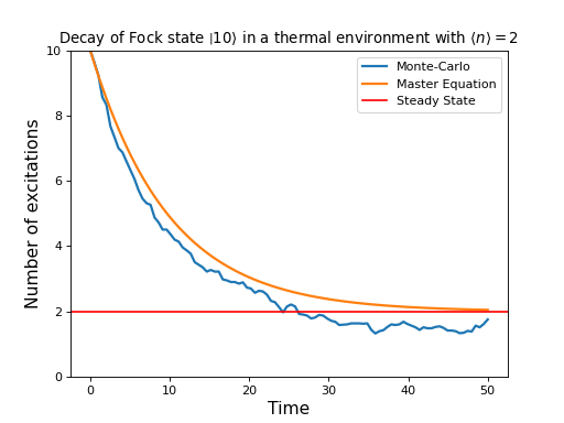
A simple example of a system that reaches a steady state is a harmonic oscillator coupled to a thermal environment. Below we consider a harmonic oscillator, initially in the \(\left|10\right>\) number state, and weakly coupled to a thermal environment characterized by an average particle expectation value of \(\left<n\right>=2\). We calculate the evolution via master equation and Monte Carlo methods, and see that they converge to the steady-state solution. Here we choose to perform only a few Monte Carlo trajectories so we can distinguish this evolution from the master-equation solution.

import numpy as np
import matplotlib.pyplot as plt

import qutip

# Define paramters
N = 20  # number of basis states to consider
a = qutip.destroy(N)
H = a.dag() * a
psi0 = qutip.basis(N, 10)  # initial state
kappa = 0.1  # coupling to oscillator

# collapse operators
c_op_list = []
n_th_a = 2  # temperature with average of 2 excitations
rate = kappa * (1 + n_th_a)
if rate > 0.0:
    c_op_list.append(np.sqrt(rate) * a)  # decay operators
rate = kappa * n_th_a
if rate > 0.0:
    c_op_list.append(np.sqrt(rate) * a.dag())  # excitation operators

# find steady-state solution
final_state = qutip.steadystate(H, c_op_list)
# find expectation value for particle number in steady state
fexpt = qutip.expect(a.dag() * a, final_state)

tlist = np.linspace(0, 50, 100)
# monte-carlo
mcdata = qutip.mcsolve(H, psi0, tlist, c_op_list, [a.dag() * a], ntraj=100)
# master eq.
medata = qutip.mesolve(H, psi0, tlist, c_op_list, [a.dag() * a])

plt.plot(tlist, mcdata.expect[0], tlist, medata.expect[0], lw=2)
# plot steady-state expt. value as horizontal line (should be = 2)
plt.axhline(y=fexpt, color='r', lw=1.5)
plt.ylim([0, 10])
plt.xlabel('Time', fontsize=14)
plt.ylabel('Number of excitations', fontsize=14)
plt.legend(('Monte-Carlo', 'Master Equation', 'Steady State'))
plt.title(
    r'Decay of Fock state $\left|10\rangle\right.$'
    r' in a thermal environment with $\langle n\rangle=2$'
)
plt.show()