Solver Class Interface
In QuTiP version 5 and later, solvers such as mesolve, mcsolve also have
a class interface. The class interface allows reusing the Hamiltonian and fine tuning
many details of how the solver is run.
Examples of some of the solver class features are given below.
Reusing Hamiltonian Data
There are many cases where one would like to study multiple evolutions of the same quantum system, whether by changing the initial state or other parameters. In order to evolve a given system as fast as possible, the solvers in QuTiP take the given input operators (Hamiltonian, collapse operators, etc) and prepare them for use with the selected ODE solver.
These operations are usually reasonably fast, but for some solvers, such as
brmesolve or fmmesolve, the overhead can be significant.
Even for simpler solvers, the time spent organizing data can become appreciable
when repeatedly solving a system.
The class interface allows us to setup the system once and reuse it with various
parameters. Most ...solve function have a paired ...Solver class, with a
..Solver.run method to run the evolution. At class
instance creation, the physics (H, c_ops, a_ops, etc.) and options
are passed. The initial state, times and expectation operators are only passed
when calling run:
times = np.linspace(0.0, 6.0, 601)
a = tensor(qeye(2), destroy(10))
sm = tensor(destroy(2), qeye(10))
e_ops = [a.dag() * a, sm.dag() * sm]
H = QobjEvo(
[a.dag()*a + sm.dag()*sm, [(sm*a.dag() + sm.dag()*a), lambda t, A: A]],
args={"A": 0.5*np.pi}
)
solver = MESolver(H, c_ops=[np.sqrt(0.1) * a], options={"atol": 1e-8})
solver.options["normalize_output"] = True
psi0 = tensor(fock(2, 0), fock(10, 5))
data1 = solver.run(psi0, times, e_ops=e_ops)
psi1 = tensor(fock(2, 0), coherent(10, 2 - 1j))
data2 = solver.run(psi1, times, e_ops=e_ops)
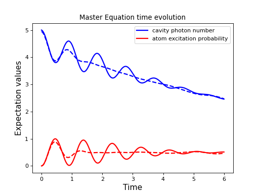
plt.figure()
plt.plot(times, data1.expect[0], "b", times, data1.expect[1], "r", lw=2)
plt.plot(times, data2.expect[0], 'b--', times, data2.expect[1], 'r--', lw=2)
plt.title('Master Equation time evolution')
plt.xlabel('Time', fontsize=14)
plt.ylabel('Expectation values', fontsize=14)
plt.legend(("cavity photon number", "atom excitation probability"))
plt.show()
Note that as shown, options can be set at initialization or with the
options property.
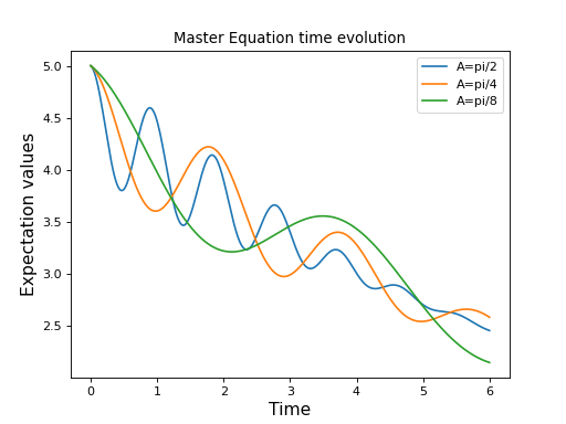
The simulation parameters, the args of the QobjEvo passed as system
operators, can be updated at the start of a run:
data1 = solver.run(psi0, times, e_ops=e_ops)
data2 = solver.run(psi0, times, e_ops=e_ops, args={"A": 0.25*np.pi})
data3 = solver.run(psi0, times, e_ops=e_ops, args={"A": 0.125*np.pi})

plt.figure()
plt.plot(times, data1.expect[0], label="A=pi/2")
plt.plot(times, data2.expect[0], label="A=pi/4")
plt.plot(times, data3.expect[0], label="A=pi/8")
plt.title('Master Equation time evolution')
plt.xlabel('Time', fontsize=14)
plt.ylabel('Expectation values', fontsize=14)
plt.legend()
plt.show()
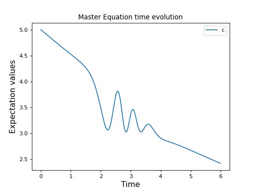
Stepping through the run
The solver class also allows to run through a simulation one step at a time, updating args at each step:
data = [5.]
solver.start(state0=psi0, t0=times[0])
for t in times[1:]:
    psi_t = solver.step(t, args={"A": np.pi*np.exp(-(t-3)**2)})
    data.append(expect(e_ops[0], psi_t))

plt.figure()
plt.plot(times, data)
plt.title('Master Equation time evolution')
plt.xlabel('Time', fontsize=14)
plt.ylabel('Expectation values', fontsize=14)
plt.legend(("cavity photon number"))
plt.show()
Note
This is an example only, updating a constant args parameter between step
should not replace using a function as QobjEvo’s coefficient.
Note
It is possible to create multiple solvers and to advance them using step in
parallel. However, many ODE solver, including the default adams method, only
allow one instance at a time per process. QuTiP supports using multiple solver instances
of these ODE solvers but with a performance cost. In these situations, using
dop853 or vern9 integration method is recommended instead.
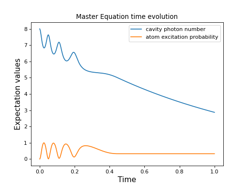
Feedback: Accessing the solver state from evolution operators
The state of the system during the evolution is accessible via properties of the solver classes.
Each solver has a StateFeedback and ExpectFeedback class method that can
be passed as arguments to time dependent systems. For example, ExpectFeedback
can be used to create a system which uncouples when there are 5 or fewer photons in the
cavity.
def f(t, e1):
    ex = (e1.real - 5)
    return (ex > 0) * ex * 10

times = np.linspace(0.0, 1.0, 301)
a  = tensor(qeye(2), destroy(10))
sm = tensor(destroy(2), qeye(10))
e_ops = [a.dag() * a, sm.dag() * sm]
psi0 = tensor(fock(2, 0), fock(10, 8))
e_ops = [a.dag() * a, sm.dag() * sm]

H = [a*a.dag(), [sm*a.dag() + sm.dag()*a, f]]
data = mesolve(H, psi0, times, c_ops=[a], e_ops=e_ops,
    args={"e1": MESolver.ExpectFeedback(a.dag() * a)}
).expect

plt.figure()
plt.plot(times, data[0])
plt.plot(times, data[1])
plt.title('Master Equation time evolution')
plt.xlabel('Time', fontsize=14)
plt.ylabel('Expectation values', fontsize=14)
plt.legend(("cavity photon number", "atom excitation probability"))
plt.show()