Superoperators, Pauli Basis and Channel Contraction
written by Christopher Granade <http://www.cgranade.com>, Institute for Quantum Computing
In this guide, we will demonstrate the tensor_contract function, which contracts one or more pairs of indices of a Qobj. This functionality can be used to find rectangular superoperators that implement the partial trace channel :math:S(rho) = Tr_2(rho)`, for instance. Using this functionality, we can quickly turn a system-environment representation of an open quantum process into a superoperator representation.
Superoperator Representations and Plotting
We start off by first demonstrating plotting of superoperators, as this will be useful to us in visualizing the results of a contracted channel.
In particular, we will use Hinton diagrams as implemented by hinton, which
show the real parts of matrix elements as squares whose size and color both correspond to the magnitude of each element. To illustrate, we first plot a few density operators.
from qutip import hinton, identity, Qobj, to_super, sigmaz, tensor, tensor_contract
from qutip.core.gates import cnot, hadamard_transform
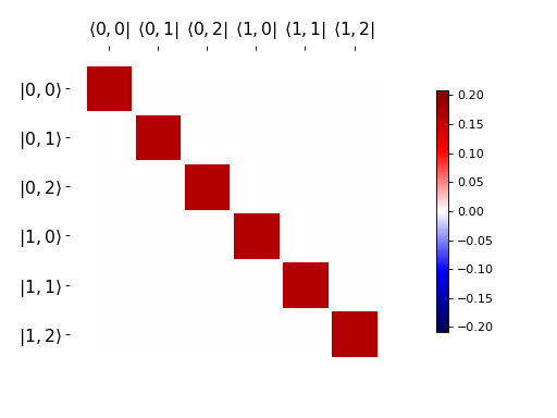
hinton(identity([2, 3]).unit())
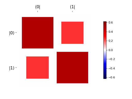
hinton(Qobj([[1, 0.5], [0.5, 1]]).unit())
We show superoperators as matrices in the Pauli basis, such that any Hermicity-preserving map is represented by a real-valued matrix. This is especially convienent for use with Hinton diagrams, as the plot thus carries complete information about the channel.
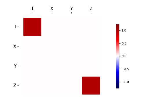
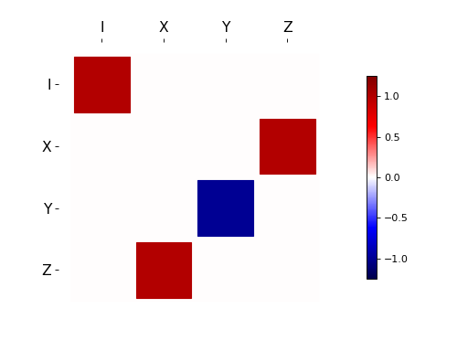
As an example, conjugation by \(\sigma_z\) leaves \(\mathbb{1}\) and \(\sigma_z\) invariant, but flips the sign of \(\sigma_x\) and \(\sigma_y\). This is indicated in Hinton diagrams by a negative-valued square for the sign change and a positive-valued square for a +1 sign.
hinton(to_super(sigmaz()))
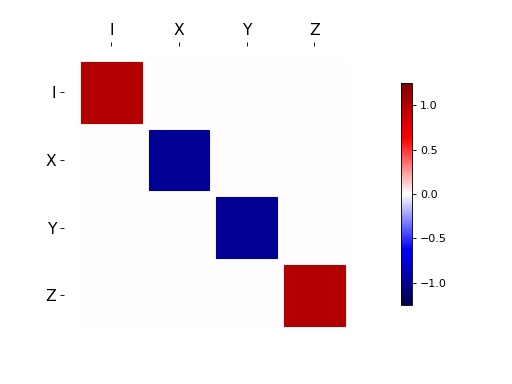
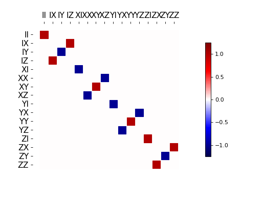
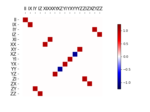
As a couple more examples, we also consider the supermatrix for a Hadamard transform and for \(\sigma_z \otimes H\).
hinton(to_super(hadamard_transform()))
hinton(to_super(tensor(sigmaz(), hadamard_transform())))
Reduced Channels
As an example of tensor contraction, we now consider the map
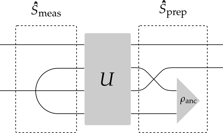
We can think of the \(\scriptstyle \rm CNOT\) here as a system-environment representation of an open quantum process, in which an environment register is prepared in a state \(\rho_{\text{anc}}\), then a unitary acts jointly on the system of interest and environment. Finally, the environment is traced out, leaving a channel on the system alone. In terms of Wood diagrams <http://arxiv.org/abs/1111.6950>, this can be represented as the composition of a preparation map, evolution under the system-environment unitary, and then a measurement map.
The integer arguments to tensor_contract address the scalar entries
of Qobj.dims after flattening the nested list from left to right. For
an ordinary operator with dims = [[a0, a1], [b0, b1]], the indices are:
index |
dimension entry |
|---|---|
|
|
|
|
|
|
|
|
Thus, tensor_contract(qobj, (1, 3)) contracts a1 with b1 and
leaves an operator with dims = [[a0], [b0]]. For superoperators, the same
rule applies to the nested dims labels passed by the user, while QuTiP
internally converts those labels to tensor axes using its column-stacking
convention. For example, to_super(identity([2, 2])).dims is
[[[2, 2], [2, 2]], [[2, 2], [2, 2]]]. In this case, index 1 is the
second output ket-space subsystem and index 3 is the matching output
bra-space subsystem.
The two tensor wires on the left indicate where we must take a tensor
contraction to obtain the measurement map. With the dims labels described
above, these are indices 1 and 3, so the corresponding
tensor_contract argument is (1, 3).
tensor_contract(to_super(identity([2, 2])), (1, 3))
Meanwhile, the super_tensor function implements the swap on the right, such that we can quickly find the preparation map.
q = tensor(identity(2), basis(2))
# now q has dims [[2, 2], [2, 1]] but we require [[2, 2], [2]]
# the following line corrects this, removing the scalar dimension
q.drop_scalar_dims(inplace=True)
s_prep = sprepost(q, q.dag())
For a \(\scriptstyle \rm CNOT\) system-environment model, the composition of these maps should give us a completely dephasing channel. The channel on both qubits is just the superunitary \(\scriptstyle \rm CNOT\) channel:
hinton(to_super(cnot()))
We now complete by multiplying the superunitary \(\scriptstyle \rm CNOT\) by the preparation channel above, then applying the partial trace channel by contracting the second and fourth index indices. As expected, this gives us a dephasing map.
hinton(tensor_contract(to_super(cnot()), (1, 3)) * s_prep)