Bosonic Environments
In this section we consider a simple two-level system coupled to a Drude-Lorentz bosonic bath. The system Hamiltonian, \(H_{sys}\), and the bath spectral density, \(J_D\), are
We will demonstrate how to describe the bath using two different expansions of the spectral density correlation function (Matsubara’s expansion and a Padé expansion), how to evolve the system in time, and how to calculate the steady state.
First we will do this in the simplest way, using the built-in implementations of
the two bath expansions, DrudeLorentzBath and
DrudeLorentzPadeBath. We will do this both with a
truncated expansion and show how to include an approximation to all of the
remaining terms in the bath expansion.
Afterwards, we will show how to calculate the bath expansion coefficients and to use those coefficients to construct your own bath description so that you can implement your own bosonic baths.
Finally, we will demonstrate how to simulate a system coupled to multiple independent baths, as occurs, for example, in certain photosynthesis processes.
A notebook containing a complete example similar to this one implemented in BoFiN can be found in example notebook 1a.
Describing the system and bath
First, let us construct the system Hamiltonian, \(H_{sys}\), and the initial
system state, rho0:
from qutip import basis, sigmax, sigmaz

# The system Hamiltonian:
eps = 0.5  # energy of the 2-level system
Del = 1.0  # tunnelling term
H_sys = 0.5 * eps * sigmaz() + 0.5 * Del * sigmax()

# Initial state of the system:
rho0 = basis(2,0) * basis(2,0).dag()
Now let us describe the bath properties:
# Bath properties:
gamma = 0.5  # cut off frequency
lam = 0.1  # coupling strength
T = 0.5  # temperature

# System-bath coupling operator:
Q = sigmaz()
where \(\gamma\) (gamma), \(\lambda\) (lam) and \(T\) are
the parameters of a Drude-Lorentz bath, and Q is the coupling operator
between the system and the bath.
We may the pass these parameters to either
DrudeLorentzBath or
DrudeLorentzPadeBath to construct an expansion of
the bath correlations:
from qutip.solver.heom import DrudeLorentzBath
from qutip.solver.heom import DrudeLorentzPadeBath

# Number of expansion terms to retain:
Nk = 2

# Matsubara expansion:
bath = DrudeLorentzBath(Q, lam, gamma, T, Nk)

# Padé expansion:
bath = DrudeLorentzPadeBath(Q, lam, gamma, T, Nk)
Where Nk is the number of terms to retain within the expansion of the
bath.
System and bath dynamics
Now we are ready to construct a solver:
from qutip.solver.heom import HEOMSolver

max_depth = 5  # maximum hierarchy depth to retain
options = {"nsteps": 15_000}

solver = HEOMSolver(H_sys, bath, max_depth=max_depth, options=options)
and to calculate the system evolution as a function of time:
tlist = [0, 10, 20]  # times to evaluate the system state at
result = solver.run(rho0, tlist)
The max_depth parameter determines how many levels of the hierarchy to
retain. As a first approximation hierarchy depth may be thought of as similar
to the order of Feynman Diagrams (both classify terms by increasing number
of interactions).
The result is a standard QuTiP results object with the attributes:
times: the times at which the state was evaluated (i.e.tlist)states: the system states at each timeexpect: a list with the values of eache_opsat each timee_data: a dictionary with the values of eache_opat each timeado_states: see below (an instance ofHierarchyADOsState)
If ado_return=True is passed to .run(...) the full set of auxilliary
density operators (ADOs) that make up the hierarchy at each time will be
returned as .ado_states. We will describe how to use these to determine
other properties, such as system-bath currents, later in the fermionic guide
(see Determining currents).
If one has a full set of ADOs from a previous call of .run(...) you may
supply it as the initial state of the solver by calling
.run(result.ado_states[-1], tlist, ado_init=True).
As with other QuTiP solvers, if expectation operators or functions are supplied
using .run(..., e_ops=[...]) the expectation values are available in
result.expect and result.e_data.
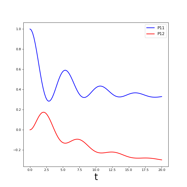
Below we run the solver again, but use e_ops to store the expectation
values of the population of the system states and the coherence:
# Define the operators that measure the populations of the two
# system states:
P11p = basis(2,0) * basis(2,0).dag()
P22p = basis(2,1) * basis(2,1).dag()

# Define the operator that measures the 0, 1 element of density matrix
# (corresonding to coherence):
P12p = basis(2,0) * basis(2,1).dag()

# Run the solver:
tlist = np.linspace(0, 20, 101)
result = solver.run(rho0, tlist, e_ops={"11": P11p, "22": P22p, "12": P12p})

# Plot the results:
fig, axes = plt.subplots(1, 1, sharex=True, figsize=(8,8))
axes.plot(result.times, result.e_data["11"], 'b', linewidth=2, label="P11")
axes.plot(result.times, result.e_data["12"], 'r', linewidth=2, label="P12")
axes.set_xlabel(r't', fontsize=28)
axes.legend(loc=0, fontsize=12)

Steady-state
Using the same solver, we can also determine the steady state of the combined system and bath using:
steady_state, steady_ados = solver.steady_state()
where steady_state is the steady state of the system and steady_ados
if the steady state of the full hierarchy. The ADO states are
described more fully in Determining currents and
HierarchyADOsState.
Matsubara Terminator
When constructing the Drude-Lorentz bath we have truncated the expansion at
Nk = 2 terms and ignore the remaining terms.
However, since the coupling to these higher order terms is comparatively weak, we may consider the interaction with them to be Markovian, and construct an additional Lindbladian term that captures their interaction with the system and the lower order terms in the expansion.
This additional term is called the terminator because it terminates the
expansion.
The DrudeLorentzBath and
DrudeLorentzPadeBath both provide a means of
calculating the terminator for a given expansion:
# Matsubara expansion:
bath = DrudeLorentzBath(Q, lam, gamma, T, Nk)

# Padé expansion:
bath = DrudeLorentzPadeBath(Q, lam, gamma, T, Nk)

# Add terminator to the system Liouvillian:
delta, terminator = bath.terminator()
HL = liouvillian(H_sys) + terminator

# Construct solver:
solver = HEOMSolver(HL, bath, max_depth=max_depth, options=options)
This captures the Markovian effect of the remaining terms in the expansion without having to fully model many more terms.
The value delta is an approximation to the strength of the effect of
the remaining terms in the expansion (i.e. how strongly the terminator is
coupled to the rest of the system).
Matsubara expansion coefficients
So far we have relied on the built-in
DrudeLorentzBath to construct the Drude-Lorentz
bath expansion for us. Now we will calculate the coefficients ourselves and
construct a BosonicBath directly. A similar
procedure can be used to apply HEOMSolver to any
bosonic bath for which we can calculate the expansion coefficients.
The real and imaginary parts of the correlation function, \(C(t)\), for the bosonic bath is expanded in an expontential series:
In the specific case of Matsubara expansion for the Drude-Lorentz bath, the coefficients of this expansion are, for the real part, \(C_{real}(t)\):
and the imaginary part, \(C_{imag}(t)\):
And now the same numbers calculated in Python:
# Convenience functions and parameters:

def cot(x):
    return 1. / np.tan(x)

beta = 1. / T

# Number of expansion terms to calculate:
Nk = 2

# C_real expansion terms:
ck_real = [lam * gamma / np.tan(gamma / (2 * T))]
ck_real.extend([
    (8 * lam * gamma * T * np.pi * k * T /
        ((2 * np.pi * k * T)**2 - gamma**2))
    for k in range(1, Nk + 1)
])
vk_real = [gamma]
vk_real.extend([2 * np.pi * k * T for k in range(1, Nk + 1)])

# C_imag expansion terms (this is the full expansion):
ck_imag = [lam * gamma * (-1.0)]
vk_imag = [gamma]
After all that, constructing the bath is very straight forward:
from qutip.solver.heom import BosonicBath

bath = BosonicBath(Q, ck_real, vk_real, ck_imag, vk_imag)
And we’re done!
The BosonicBath can be used with the
HEOMSolver in exactly the same way as the baths
we constructed previously using the built-in Drude-Lorentz bath expansions.
Multiple baths
The HEOMSolver supports having a system interact
with multiple environments. All that is needed is to supply a list of baths
instead of a single bath.
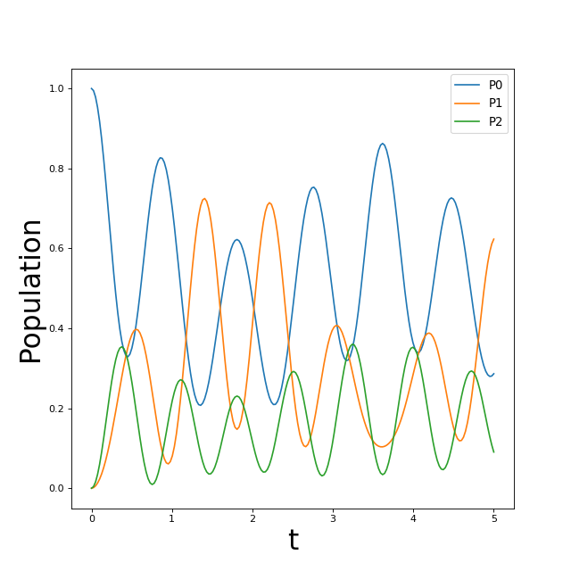
In the example below we calculate the evolution of a small system where each basis state of the system interacts with a separate bath. Such an arrangement can model, for example, the Fenna–Matthews–Olson (FMO) pigment-protein complex which plays an important role in photosynthesis ( for a full FMO example see the notebook https://github.com/tehruhn/bofin/blob/main/examples/example-2-FMO-example.ipynb ).
For each bath expansion, we also include the terminator in the system Liouvillian.
At the end, we plot the populations of the system states as a function of time, and show the long-time beating of quantum state coherence that occurs:
# The size of the system:
N_sys = 3

def proj(i, j):
    """ A helper function for creating an interaction operator. """
    return basis(N_sys, i) * basis(N_sys, j).dag()

# Construct one bath for each system state:
baths = []
for i in range(N_sys):
    Q = proj(i, i)
    baths.append(DrudeLorentzBath(Q, lam, gamma, T, Nk))

# Construct the system Liouvillian from the system Hamiltonian and
# bath expansion terminators:
H_sys = sum((i + 0.5) * eps * proj(i, i) for i in range(N_sys))
H_sys += sum(
  (i + j + 0.5) * Del * proj(i, j)
  for i in range(N_sys) for j in range(N_sys)
  if i != j
)
HL = liouvillian(H_sys) + sum(bath.terminator()[1] for bath in baths)

# Construct the solver (pass a list of baths):
solver = HEOMSolver(HL, baths, max_depth=max_depth, options=options)

# Run the solver:
rho0 = basis(N_sys, 0) * basis(N_sys, 0).dag()
tlist = np.linspace(0, 5, 200)
e_ops = {
    f"P{i}": proj(i, i)
    for i in range(N_sys)
}
result = solver.run(rho0, tlist, e_ops=e_ops)

# Plot populations:
fig, axes = plt.subplots(1, 1, sharex=True, figsize=(8,8))
for label, values in result.e_data.items():
    axes.plot(result.times, values, label=label)
axes.set_xlabel(r't', fontsize=28)
axes.set_ylabel(r"Population", fontsize=28)
axes.legend(loc=0, fontsize=12)
