Fermionic Environments
Here we model a single fermion coupled to two electronic leads or reservoirs (e.g., this can describe a single quantum dot, a molecular transistor, etc). The system hamiltonian, \(H_{sys}\), and bath spectral density, \(J_D\), are
We will demonstrate how to describe the bath using two different expansions of the spectral density correlation function (Matsubara’s expansion and a Padé expansion), how to evolve the system in time, and how to calculate the steady state.
Since our fermion is coupled to two reservoirs, we will construct two baths – one for each reservoir or lead – and call them the left (L) and right (R) baths for convenience. Each bath will have a different chemical potential \(\mu\) which we will label \(\mu_L\) and \(\mu_R\).
First we will do this using the built-in implementations of the bath expansions,
LorentzianBath and
LorentzianPadeBath.
Afterwards, we will show how to calculate the bath expansion coefficients and to
use those coefficients to construct your own bath description so that you can
implement your own fermionic baths.
Environment API
As for the bosonic case, we will include brief intermissions showing how to achieve the same results using the newer environment API. The “bath” classes are part of an older API that is less powerful, but often more convenient to use when one only uses the HEOM solver and does not need any of the new features.
Our implementation of fermionic baths primarily follows the definitions used in the dissertation of Christian Schinabeck and related publications. A notebook containing a complete example similar to this one implemented in BoFiN can be found in HEOM example notebook 5a.
Describing the system and bath
First, let us construct the system Hamiltonian, \(H_{sys}\), and the initial
system state, rho0:
from qutip import basis, destroy

# The system Hamiltonian:
e1 = 1.  # site energy
H_sys = e1 * destroy(2).dag() * destroy(2)

# Initial state of the system:
rho0 = basis(2,0) * basis(2,0).dag()
Now let us describe the bath properties:
# Shared bath properties:
gamma = 0.01     # coupling strength
W = 1.0          # cut-off
T = 0.025851991  # temperature
beta = 1. / T

# Chemical potentials for the two baths:
mu_L = 1.
mu_R = -1.

# System-bath coupling operator:
Q = destroy(2)
where \(\Gamma\) (gamma), \(W\) and the temperature \(T\) are the parameters of
an Lorentzian bath, \(\mu_L\) (mu_L) and \(\mu_R\) (mu_R) are
the chemical potentials of the left and right baths, and Q is the coupling
operator between the system and the baths. QuTiP assumes a number-conserving coupling term, as described
in the section on fermionic environments.
We may the pass these parameters to either LorentzianBath or
LorentzianPadeBath to construct an expansion of the bath correlations:
from qutip.solver.heom import LorentzianBath
from qutip.solver.heom import LorentzianPadeBath

# Number of expansion terms to retain:
Nk = 2

# Matsubara expansion:
bath_L = LorentzianBath(Q, gamma, W, mu_L, T, Nk, tag="L")
bath_R = LorentzianBath(Q, gamma, W, mu_R, T, Nk, tag="R")

# Padé expansion:
bath_L = LorentzianPadeBath(Q, gamma, W, mu_L, T, Nk, tag="L")
bath_R = LorentzianPadeBath(Q, gamma, W, mu_R, T, Nk, tag="R")
Here, Nk is the number of terms to retain within the expansion of the bath.
Note that we haved labelled each bath with a tag (either “L” or “R”) so that we can identify the exponents from individual baths later when calculating the currents between the system and the bath.
Environment API
In analogy to the Drude-Lorentz environment in the previous section,
we first create a LorentzianEnvironment that describes the bath abstractly
and then invoke approximation methods:
from qutip.core.environment import LorentzianEnvironment

env_L = LorentzianEnvironment(T, mu_L, gamma, W)
env_R = LorentzianEnvironment(T, mu_R, gamma, W)

# Matsubara expansion:
approx_L = env_L.approx_by_matsubara(Nk, tag="L")
approx_R = env_R.approx_by_matsubara(Nk, tag="R")

# Pade expansion:
approx_L = env_L.approx_by_pade(Nk, tag="L")
approx_R = env_R.approx_by_pade(Nk, tag="R")
System and bath dynamics
Now we are ready to construct a solver:
from qutip.solver.heom import HEOMSolver

max_depth = 5  # maximum hierarchy depth to retain
options = {"nsteps": 15_000}
baths = [bath_L, bath_R]

solver = HEOMSolver(H_sys, baths, max_depth=max_depth, options=options)
and to calculate the system evolution as a function of time:
tlist = [0, 10, 20]  # times to evaluate the system state at
result = solver.run(rho0, tlist)
As in the bosonic case, the max_depth parameter determines how many levels
of the hierarchy to retain.
Also here, we can specify e_ops in order to retrieve the
expectation values of operators at each given time. See
the previous section for a fuller description of
the returned result object.
Environment API
When using the environment API, we again have to pass the coupling operator to the HEOM solver together with the approximated environment:
solver = HEOMSolver(H_sys, [(approx_L, Q), (approx_R, Q)],
                    max_depth=max_depth, options=options)
Below we run the solver again, but use e_ops to store the expectation
values of the population of the system states:
# Define the operators that measure the populations of the two
# system states:
P11p = basis(2,0) * basis(2,0).dag()
P22p = basis(2,1) * basis(2,1).dag()

# Run the solver:
tlist = np.linspace(0, 500, 101)
result = solver.run(rho0, tlist, e_ops={"11": P11p, "22": P22p})

# Plot the results:
fig, axes = plt.subplots(1, 1, sharex=True, figsize=(6, 6))
axes.plot(result.times, np.real(result.e_data["11"]), 'b', linewidth=2, label="P11")
axes.plot(result.times, np.real(result.e_data["22"]), 'r', linewidth=2, label="P22")
axes.set_xlabel(r't', fontsize=16)
axes.legend(loc=0, fontsize=16)
The plot above is not very exciting. What we would really like to see in this case are the currents between the system and the two baths. We will plot these in the next section using the auxiliary density operators (ADOs) returned by the solver.
Determining currents
The currents between the system and a fermionic bath may be calculated from the first level auxiliary density operators (ADOs) associated with the exponents of that bath.
The contribution to the current into a given bath from each exponent in that bath is:
where the \(\pm\) sign depends on whether the exponent corresponds to the \(C^+(t)\) or the \(C^-(t)\) correlation function
(see the explanation in the guide on Fermionic Environments) and
\(Q^\pm\) is \(Q\) for + exponents and \(Q^{\dagger}\) for - exponents.
The first-level exponents for the left bath are retrieved by calling
.filter(tags=["L"]) on ado_state which is an instance of
HierarchyADOsState and also provides access to
the methods of HierarchyADOs which describes the
structure of the hierarchy for a given problem.
Here the tag “L” matches the tag passed when constructing bath_L earlier
in this example.
Similarly, we may calculate the current to the right bath from the exponents tagged with “R”.
def exp_current(aux, exp):
    """ Calculate the current for a single exponent. """
    sign = 1 if exp.type == exp.types["+"] else -1
    op = exp.Q if exp.type == exp.types["+"] else exp.Q.dag()
    return 1j * sign * (op * aux).tr()

def heom_current(tag, ado_state):
    """ Calculate the current between the system and the given bath. """
    level_1_ados = [
        (ado_state.extract(label), ado_state.exps(label)[0])
        for label in ado_state.filter(tags=[tag])
    ]
    return np.real(sum(exp_current(aux, exp) for aux, exp in level_1_ados))

heom_left_current = lambda t, ado_state: heom_current("L", ado_state)
heom_right_current = lambda t, ado_state: heom_current("R", ado_state)
Once we have defined functions for retrieving the currents for the
baths, we can pass them to e_ops and plot the results:
# Run the solver (returning ADO states):
tlist = np.linspace(0, 100, 201)
result = solver.run(rho0, tlist, e_ops={
    "left_currents": heom_left_current,
    "right_currents": heom_right_current,
})

# Plot the results:
fig, axes = plt.subplots(1, 1, sharex=True, figsize=(8,8))
axes.plot(
    result.times, result.e_data["left_currents"], 'b',
    linewidth=2, label=r"Bath L",
)
axes.plot(
    result.times, result.e_data["right_currents"], 'r',
    linewidth=2, label="Bath R",
)
axes.set_xlabel(r't', fontsize=16)
axes.set_ylabel(r'Current', fontsize=16)
axes.set_title(r'System to Bath Currents', fontsize=16)
axes.legend(loc=0, fontsize=16)

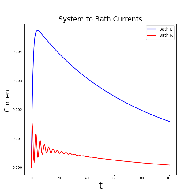
And now we have a more interesting plot that shows the currents to the left and right baths decaying towards their steady states!
In the next section, we will calculate the steady state currents directly.
Steady state currents
Using the same solver, we can also determine the steady state of the combined system and bath using:
steady_state, steady_ados = solver.steady_state()
and calculate the steady state currents to the two baths from steady_ados
using the same heom_current function we defined previously:
steady_state_current_left = heom_current("L", steady_ados)
steady_state_current_right = heom_current("R", steady_ados)
Now we can add the steady state currents to the previous plot:
# Plot the results and steady state currents:
fig, axes = plt.subplots(1, 1, sharex=True, figsize=(8,8))
axes.plot(
    result.times, result.e_data["left_currents"], 'b',
    linewidth=2, label=r"Bath L",
)
axes.plot(
    result.times, [steady_state_current_left] * len(result.times), 'b:',
    linewidth=2, label=r"Bath L (steady state)",
)
axes.plot(
    result.times, result.e_data["right_currents"], 'r',
    linewidth=2, label="Bath R",
)
axes.plot(
    result.times, [steady_state_current_right] * len(result.times), 'r:',
    linewidth=2, label=r"Bath R (steady state)",
)
axes.set_xlabel(r't', fontsize=28)
axes.set_ylabel(r'Current', fontsize=20)
axes.set_title(r'System to Bath Currents (with steady states)', fontsize=20)
axes.legend(loc=0, fontsize=12)

As you can see, there is still some way to go beyond t = 100 before the
steady state is reached!
Padé expansion coefficients
As in the bosonic case, we can also use manually calculated correlation function coefficients of fermionic environments with the HEOM solver. In the section on fermionic environments, we defined their correlation functions and calculated the Matsubara and Pade expansions for Lorentzian environments.
For the Lorentzian bath, the Padé expansion converges much more quickly, so we will calculate the Padé expansion coefficients here. In Python code, the calculation can be done as follows:
# Imports
from numpy.linalg import eigvalsh

# Convenience functions and parameters:
def deltafun(j, k):
    """ Kronecker delta function. """
    return 1.0 if j == k else 0.

def f_approx(x, Nk):
    """ Padé approxmation to Fermi distribution. """
    f = 0.5
    for ll in range(1, Nk + 1):
        # kappa and epsilon are calculated further down
        f = f - 2 * kappa[ll] * x / (x**2 + epsilon[ll]**2)
    return f

def kappa_epsilon(Nk):
    """ Calculate kappa and epsilon coefficients. """

    alpha = np.zeros((2 * Nk, 2 * Nk))
    for j in range(2 * Nk):
        for k in range(2 * Nk):
            alpha[j][k] = (
                (deltafun(j, k + 1) + deltafun(j, k - 1))
                / np.sqrt((2 * (j + 1) - 1) * (2 * (k + 1) - 1))
            )

    eps = [-2. / val for val in eigvalsh(alpha)[:Nk]]

    alpha_p = np.zeros((2 * Nk - 1, 2 * Nk - 1))
    for j in range(2 * Nk - 1):
        for k in range(2 * Nk - 1):
            alpha_p[j][k] = (
                (deltafun(j, k + 1) + deltafun(j, k - 1))
                / np.sqrt((2 * (j + 1) + 1) * (2 * (k + 1) + 1))
            )

    chi = [-2. / val for val in eigvalsh(alpha_p)[:Nk - 1]]

    eta_list = [
        0.5 * Nk * (2 * (Nk + 1) - 1) * (
            np.prod([chi[k]**2 - eps[j]**2 for k in range(Nk - 1)]) /
            np.prod([
                eps[k]**2 - eps[j]**2 + deltafun(j, k) for k in range(Nk)
            ])
        )
        for j in range(Nk)
    ]

    kappa = [0] + eta_list
    epsilon = [0] + eps

    return kappa, epsilon

kappa, epsilon = kappa_epsilon(Nk)

# Phew, we made it to function that calculates the coefficients for the
# correlation function expansions:

def C(sigma, mu, Nk):
    r""" Calculate the expansion coefficients for C_\sigma. """
    beta = 1. / T
    ck = [0.5 * gamma * W * f_approx(1.0j * beta * W, Nk)]
    vk = [W - sigma * 1.0j * mu]
    for ll in range(1, Nk + 1):
        ck.append(
            -1.0j * (kappa[ll] / beta) * gamma * W**2
            / (-(epsilon[ll]**2 / beta**2) + W**2)
        )
        vk.append(epsilon[ll] / beta - sigma * 1.0j * mu)
    return ck, vk

ck_plus_L, vk_plus_L = C(1.0, mu_L, Nk)  # C_+, left bath
ck_minus_L, vk_minus_L = C(-1.0, mu_L, Nk)  # C_-, left bath

ck_plus_R, vk_plus_R = C(1.0, mu_R, Nk)  # C_+, right bath
ck_minus_R, vk_minus_R = C(-1.0, mu_R, Nk)  # C_-, right bath
Finally we are ready to construct the
FermionicBath:
from qutip.solver.heom import FermionicBath

# Padé expansion:
bath_L = FermionicBath(Q, ck_plus_L, vk_plus_L, ck_minus_L, vk_minus_L)
bath_R = FermionicBath(Q, ck_plus_R, vk_plus_R, ck_minus_R, vk_minus_R)
And we’re done!
The FermionicBath can be used with the
HEOMSolver in exactly the same way as the baths
we constructed previously using the built-in Lorentzian bath expansions.
Environment API
The analogue of the FermionicBath is the ExponentialFermionicEnvironment.
Its usage is very similar:
from qutip.core.environment import ExponentialFermionicEnvironment

env_L = ExponentialFermionicEnvironment(ck_plus_L, vk_plus_L, ck_minus_L, vk_minus_L)
env_R = ExponentialFermionicEnvironment(ck_plus_R, vk_plus_R, ck_minus_R, vk_minus_R)