Krylov Solver

The Krylov Subspace Method

To approximate quantum dynamics in systems with a high number of degrees of freedom, the Krylov-subspace method is a standard method for efficient calculation. Let \(\left|\psi\right\rangle\) be a state in a \(D\)-dimensional complex Hilbert space that evolves under a time-independent Hamiltonian \(H\). Then, the \(N\)-dimensional Krylov subspace associated with that state and Hamiltonian is given by

(1)\[\mathcal{K}_{N}=\operatorname{span}\left\{|\psi\rangle, H|\psi\rangle, \ldots, H^{N-1}|\psi\rangle\right\},\]

where the dimension \(N<D\) is a parameter of choice. To construct an orthonormal basis \(B_N\) for \(\mathcal{K}_{N}\), the simplest algorithm is the well-known Lanczos algorithm, which provides a sort of Gram-Schmidt procedure. Written in this basis the time-evolved state can be approximated as

(2)\[|\psi(t)\rangle=e^{-iHt}|\psi\rangle\approx\mathbb{P}_{N}e^{-iHt}\mathbb{P}_{N}|\psi\rangle=\mathbb{V}_{N}^{\dagger}e^{-iT_{N}t}\mathbb{V}_{N}|\psi\rangle\equiv\left|\psi_{N}(t)\right\rangle,\]

where \(T_{N}=\mathbb{V}_{N} H \mathbb{V}_{N}^{\dagger}\) is the Hamiltonian reduced to the Krylov subspace (which takes a tridiagonal matrix form), and \(\mathbb{V}_{N}^{\dagger}\) is the matrix containing the vectors of the Krylov basis as columns.

With the above approximation, the time-evolution is calculated only with a smaller square matrix of the desired size. Therefore, the Krylov method provides huge speed-ups in computation of short-time evolutions when the dimension of the Hamiltonian is very large, a point at which exact calculations on the complete subspace are practically impossible.

One of the biggest problems with this type of method is the control of the error. After a short time, the error starts to grow exponentially. However, this can be easily corrected by restarting the subspace when the error reaches a certain threshold. Therefore, a series of \(M\) Krylov-subspace time evolutions provides accurate solutions for the complete time evolution. Within this scheme, the magic of Krylov resides not only in its ability to capture complex time evolutions from very large Hilbert spaces with very small dimenions \(M\), but also in the computing speed-up it presents.

For exceptional cases, the Lanczos algorithm might arrive at the exact evolution of the initial state at a dimension \(M_{hb}<M\). This is called a happy breakdown. For example, if a Hamiltonian has a symmetry subspace \(D_{\text{sim}}<M\), then the algorithm will optimize using the value math:M_{hb}<M:, at which the evolution is not only exact but also cheap.

Krylov for Mixed States

In a similar manner, the Liouvillian \(\mathcal{L}\) of a system can be taken as in input for the construction of the Kyrlov basis. This extends the applicability of this method to density operator dyanmics in both closed and open systems. In these cases, the subspace is spanned by repeated application of the Liouvillian onto the vectorized form of the density operator, thereby forming

(3)\[\mathcal{K}_{N}=\operatorname{span}\left\{|\rho), H|\psi\rangle, \ldots, \mathcal{L}^{N-1}|\psi\rangle\right\}.\]

Same as for the pure states mentioned above, the Krylov basis vectors are calculated using the Lanczos algorithm (or alternative - see below).

Alternative Algorithms for Kyrlov Construction

As the number of degrees of freedom grows, the standard Lanczos algorithm shows significant errors due to numerical inaccuracies. This is why the default algorithm in QuTiP to construct the Krylov basis is the fully-reorthogonalized Lanczos algorithm (FRO). It orthogonalizes new basis vectors with respect to all (contrary to just the last two) previously created vectors to greatly limit the accumulation of numerical errors. However, by specifically setting options["algorithm"]="lanczos", the standard Lanczos algorithm is still available.

In addition, QuTiP supports the Arnoldi iteration. It is necessary to correctly calculate open system dynamics. Contrary to the standard Lanczos and FRO Lanczos which produce a tri-diagonal matrix, the Arnoldi interation provides an upper-Hessenberg form.

Finding a Good Krylov-Subspace Dimension

With the Krylov-subspace method, great computational speed-ups can be achieved especially for large systems and short time evolutions. In QuTiP, the integrator calculates the subspace up to the parameter krylov_dim (or until a happy breakdown is detected). It then evolves the state up to the time where accuracy up to the provided tolerance atol is still guaranteed, and then recalculates the subspace. By repeating this, the time evolution is calculated.

To achieve the promised speed-up, it is essential to choose a suitable Krylov-subspace dimension. Too small a dimension leads to frequent recalculation of the Kyrlov basis and thus high computational load. Too big of a basis however leads to an increasingly expensive calculation of basis vectors and little gain in accuracy.

Therefore, aiming for a Krylov-dimension that is much smaller than the provided Hilbert space (or Liouvillian space) is recommended. However, the optimal dimension very much depends on both the Hamiltonian and the initial state.

Krylov Solver in QuTiP

In QuTiP, Krylov-subspace evolution is implemented as the function krylovsolve. Arguments are nearly the same as sesolve or mesolve function for master-equation evolution, except that the Hamiltonian cannot depend on time and an additional parameter krylov_dim is needed. krylov_dim defines the maximum allowed Krylov-subspace dimension.

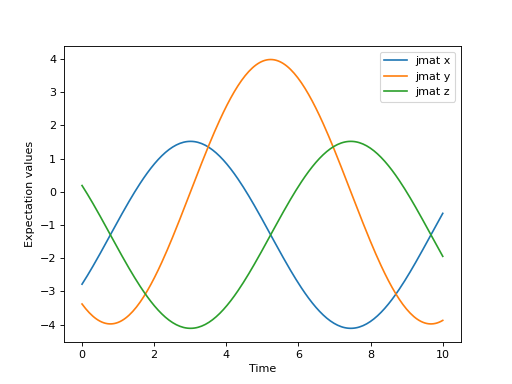
Let’s solve a simple example using the algorithm in QuTiP to get familiar with the method.

>>> dim = 100
>>> jx = jmat((dim - 1) / 2.0, "x")
>>> jy = jmat((dim - 1) / 2.0, "y")
>>> jz = jmat((dim - 1) / 2.0, "z")
>>> e_ops = [jx, jy, jz]
>>> H = (jz + jx) / 2
>>> psi0 = rand_ket(dim, seed=1)
>>> tlist = np.linspace(0.0, 10.0, 200)
>>> results = krylovsolve(H, psi0, tlist, krylov_dim=20, e_ops=e_ops)
>>> plt.figure()
>>> for expect in results.expect:
>>>    plt.plot(tlist, expect)
>>> plt.legend(('jmat x', 'jmat y', 'jmat z'))
>>> plt.xlabel('Time')
>>> plt.ylabel('Expectation values')
>>> plt.show()