Monte Carlo for Non-Markovian Dynamics

The Monte Carlo solver of QuTiP can also be used to solve the dynamics of time-local non-Markovian master equations, i.e., master equations of the Lindblad form

(1)\[\dot\rho(t) = -\frac{i}{\hbar} [H, \rho(t)] + \sum_n \frac{\gamma_n(t)}{2} \left[2 A_n \rho(t) A_n^\dagger - \rho(t) A_n^\dagger A_n - A_n^\dagger A_n \rho(t)\right]\]

with “rates” \(\gamma_n(t)\) that can take negative values. This can be done with the nm_mcsolve function. The function is based on the influence martingale formalism [Donvil22] and formally requires that the collapse operators \(A_n\) satisfy a completeness relation of the form

(2)\[\sum_n A_n^\dagger A_n = \alpha \mathbb{I} ,\]

where \(\mathbb{I}\) is the identity operator on the system Hilbert space and \(\alpha>0\). Note that when the collapse operators of a model don’t satisfy such a relation, nm_mcsolve automatically adds an extra collapse operator such that (2) is satisfied. The rate corresponding to this extra collapse operator is set to zero.

Technically, the influence martingale formalism works as follows. We introduce an influence martingale \(\mu(t)\), which follows the evolution of the system state. When no jump happens, it evolves as

(3)\[\mu(t) = \exp\left( \alpha\int_0^t K(\tau) d\tau \right)\]

where \(K(t)\) is for now an arbitrary function. When a jump corresponding to the collapse operator \(A_n\) happens, the influence martingale becomes

(4)\[\mu(t+\delta t) = \mu(t)\left(\frac{K(t)-\gamma_n(t)}{\gamma_n(t)}\right)\]

Assuming that the state \(\bar\rho(t)\) computed by the Monte Carlo average

(5)\[\bar\rho(t) = \frac{1}{N}\sum_{l=1}^N |\psi_l(t)\rangle\langle \psi_l(t)|\]

solves a Lindblad master equation with collapse operators \(A_n\) and rates \(\Gamma_n(t)\), the state \(\rho(t)\) defined by

(6)\[\rho(t) = \frac{1}{N}\sum_{l=1}^N \mu_l(t) |\psi_l(t)\rangle\langle \psi_l(t)|\]

solves a Lindblad master equation with collapse operators \(A_n\) and shifted rates \(\gamma_n(t)-K(t)\). Thus, while \(\Gamma_n(t) \geq 0\), the new “rates” \(\gamma_n(t) = \Gamma_n(t) - K(t)\) satisfy no positivity requirement.

The input of nm_mcsolve is almost the same as for mcsolve. The only difference is how the collapse operators and rate functions should be defined. nm_mcsolve requires collapse operators \(A_n\) and target “rates” \(\gamma_n\) (which are allowed to take negative values) to be given in list form [[C_1, gamma_1], [C_2, gamma_2], ...]. Note that we give the actual rate and not its square root, and that nm_mcsolve automatically computes associated jump rates \(\Gamma_n(t)\geq0\) appropriate for simulation.

We conclude with a simple example demonstrating the usage of the nm_mcsolve function. For more elaborate, physically motivated examples, we refer to the accompanying tutorial notebook.

times = np.linspace(0, 1, 201)
psi0 = basis(2, 1)
a0 = destroy(2)
H = a0.dag() * a0

# Rate functions
gamma1 = "kappa * nth"
gamma2 = "kappa * (nth+1) + 12 * np.exp(-2*t**3) * (-np.sin(15*t)**2)"
# gamma2 becomes negative during some time intervals

# nm_mcsolve integration
ops_and_rates = []
ops_and_rates.append([a0.dag(), gamma1])
ops_and_rates.append([a0,       gamma2])
MCSol = nm_mcsolve(H, psi0, times, ops_and_rates,
                   args={'kappa': 1.0 / 0.129, 'nth': 0.063},
                   e_ops=[a0.dag() * a0, a0 * a0.dag()],
                   options={'map': 'parallel'}, ntraj=2500)

# mesolve integration for comparison
d_ops = [[lindblad_dissipator(a0.dag(), a0.dag()), gamma1],
         [lindblad_dissipator(a0, a0),             gamma2]]
MESol = mesolve(H, psi0, times, d_ops, e_ops=[a0.dag() * a0, a0 * a0.dag()],
                args={'kappa': 1.0 / 0.129, 'nth': 0.063})

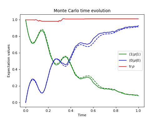
plt.figure()
plt.plot(times, MCSol.expect[0], 'g',
         times, MCSol.expect[1], 'b',
         times, MCSol.trace, 'r')
plt.plot(times, MESol.expect[0], 'g--',
         times, MESol.expect[1], 'b--')
plt.title('Monte Carlo time evolution')
plt.xlabel('Time')
plt.ylabel('Expectation values')
plt.legend((r'$\langle 1 | \rho | 1 \rangle$',
            r'$\langle 0 | \rho | 0 \rangle$',
            r'$\operatorname{tr} \rho$'))
plt.show()