Solving Problems with Time-dependent Hamiltonians

Time-Dependent Operators

In the previous examples of quantum evolution, we assumed that the systems under consideration were described by time-independent Hamiltonians. However, many systems have explicit time dependence in either the Hamiltonian, or the collapse operators describing coupling to the environment, and sometimes both components might depend on time. The time-evolutions solvers such as sesolve, brmesolve, etc. are all capable of handling time-dependent Hamiltonians and collapse terms. QuTiP use QobjEvo to represent time-dependent quantum operators. There are three different ways to build a QobjEvo:

1. Function based: Build the time dependent operator from a function returning a Qobj:

def oper(t):
    return num(N) + (destroy(N) + create(N)) * np.sin(t)

H_t = QobjEvo(oper)

1. List based: The time dependent quantum operator is represented as a list of qobj and [qobj, coefficient] pairs:

H_t = QobjEvo([num(N), [create(N), lambda t: np.sin(t)], [destroy(N), lambda t: np.sin(t)]])

3. coefficent based: The product of a Qobj with a Coefficient, created by the coefficient function, result in a QobjEvo:

coeff = coefficent(lambda t: np.sin(t))
H_t = num(N) + (destroy(N) + create(N)) * coeff

These 3 examples will create the same time dependent operator, however the function based method will usually be slower when used in solver.

Most solvers accept a QobjEvo when an operator is expected: this include the Hamiltonian H, collapse operators, expectation values operators, the operator of brmesolve’s a_ops, etc. Exception are krylovsolve’s Hamiltonian and HEOM’s Bath operators.

Most solvers will accept any format that could be made into a QobjEvo for the Hamiltonian. All of the following are equivalent:

result = mesolve(H_t, ...)
result = mesolve([num(N), [destroy(N) + create(N), lambda t: np.sin(t)]], ...)
result = mesolve(oper, ...)

Collapse operator also accept a list of object that could be made into QobjEvo. However one needs to be careful about not confusing the list nature of the c_ops parameter with list format quantum system. In the following call:

result = mesolve(H_t, ..., c_ops=[num(N), [destroy(N) + create(N), lambda t: np.sin(t)]])

mesolve will see 2 collapses operators: num(N) and [destroy(N) + create(N), lambda t: np.sin(t)]. It is therefore preferred to pass each collapse operator as either a Qobj or a QobjEvo.

As an example, we will look at a case with a time-dependent Hamiltonian of the form \(H=H_{0}+f(t)H_{1}\) where \(f(t)\) is the time-dependent driving strength given as \(f(t)=A\exp\left[-\left( t/\sigma \right)^{2}\right]\). The following code sets up the problem

ustate = basis(3, 0)
excited = basis(3, 1)
ground = basis(3, 2)

N = 2 # Set where to truncate Fock state for cavity
sigma_ge = tensor(qeye(N), ground * excited.dag())  # |g><e|
sigma_ue = tensor(qeye(N), ustate * excited.dag())  # |u><e|
a = tensor(destroy(N), qeye(3))
ada = tensor(num(N), qeye(3))

c_ops = []  # Build collapse operators
kappa = 1.5 # Cavity decay rate
c_ops.append(np.sqrt(kappa) * a)
gamma = 6  # Atomic decay rate
c_ops.append(np.sqrt(5*gamma/9) * sigma_ue) # Use Rb branching ratio of 5/9 e->u
c_ops.append(np.sqrt(4*gamma/9) * sigma_ge) # 4/9 e->g

t = np.linspace(-15, 15, 100) # Define time vector
psi0 = tensor(basis(N, 0), ustate) # Define initial state

state_GG = tensor(basis(N, 1), ground) # Define states onto which to project
sigma_GG = state_GG * state_GG.dag()
state_UU = tensor(basis(N, 0), ustate)
sigma_UU = state_UU * state_UU.dag()

g = 5  # coupling strength
H0 = -g * (sigma_ge.dag() * a + a.dag() * sigma_ge)  # time-independent term
H1 = (sigma_ue.dag() + sigma_ue)  # time-dependent term

Given that we have a single time-dependent Hamiltonian term, and constant collapse terms, we need to specify a single Python function for the coefficient \(f(t)\). In this case, one can simply do

def H1_coeff(t):
    return 9 * np.exp(-(t / 5.) ** 2)

In this case, the return value depends only on time. However it is possible to add optional arguments to the call, see Using arguments. Having specified our coefficient function, we can now specify the Hamiltonian in list format and call the solver (in this case mesolve)

H = [H0, [H1, H1_coeff]]
output = mesolve(H, psi0, t, c_ops, [ada, sigma_UU, sigma_GG])

We can call the Monte Carlo solver in the exact same way (if using the default ntraj=500):

output = mcsolve(H, psi0, t, c_ops, [ada, sigma_UU, sigma_GG])

The output from the master equation solver is identical to that shown in the examples, the Monte Carlo however will be noticeably off, suggesting we should increase the number of trajectories for this example. In addition, we can also consider the decay of a simple Harmonic oscillator with time-varying decay rate

kappa = 0.5

def col_coeff(t, args):  # coefficient function
    return np.sqrt(kappa * np.exp(-t))

N = 10  # number of basis states
a = destroy(N)
H = a.dag() * a  # simple HO
psi0 = basis(N, 9)  # initial state
c_ops = [QobjEvo([a, col_coeff])]  # time-dependent collapse term
times = np.linspace(0, 10, 100)
output = mesolve(H, psi0, times, c_ops, [a.dag() * a])

Qobjevo

QobjEvo as a time dependent quantum system, as it’s main functionality create a Qobj at a time:

>>> print(H_t(np.pi / 2))
Quantum object: dims=[[2], [2]], shape=(2, 2), type='oper', isherm=True
Qobj data =
[[0. 1.]
 [1. 1.]]

QobjEvo shares a lot of properties with the Qobj.

Property	Attribute	Description
Dimensions	Q.dims	Shapes the tensor structure.
Shape	Q.shape	Dimensions of underlying data matrix.
Type	Q.type	Is object of type ‘ket, ‘bra’, ‘oper’, or ‘super’?
Representation	Q.superrep	Representation used if type is ‘super’?
Is constant	Q.isconstant	Does the QobjEvo depend on time.

QobjEvo’s follow the same mathematical operations rules than Qobj. They can be added, subtracted and multiplied with scalar, Qobj and QobjEvo. They also support the dag and trans and conj method and can be used for tensor operations and super operator transformation:

H = tensor(H_t, qeye(2))
c_op = tensor(QobjEvo([destroy(N), lambda t: np.exp(-t)]), sigmax())

L = -1j * (spre(H) - spost(H.dag()))
L += spre(c_op) * spost(c_op.dag()) - 0.5 * spre(c_op.dag() * c_op) - 0.5 * spost(c_op.dag() * c_op)

Or equivalently:

L = liouvillian(H, [c_op])

Using arguments

Until now, the coefficients were only functions of time. In the definition of H1_coeff, the driving amplitude A and width sigma were hardcoded with their numerical values. This is fine for problems that are specialized, or that we only want to run once. However, in many cases, we would like study the same problem with a range of parameters and not have to worry about manually changing the values on each run. QuTiP allows you to accomplish this using by adding extra arguments to coefficients function that make the QobjEvo. For instance, instead of explicitly writing 9 for the amplitude and 5 for the width of the gaussian driving term, we can add an args positional variable:

>>> def H1_coeff(t, args):
>>>     return args['A'] * np.exp(-(t/args['sigma'])**2)

or, new from v5, add the extra parameter directly:

>>> def H1_coeff(t, A, sigma):
>>>     return A * np.exp(-(t / sigma)**2)

When the second positional input of the coefficient function is named args, the arguments are passed as a Python dictionary of key: value pairs. Otherwise the coefficient function is called as coeff(t, **args). In the last example, args = {'A': a, 'sigma': b} where a and b are the two parameters for the amplitude and width, respectively. This args dictionary need to be given at creation of the QobjEvo when function using then are included:

>>> system = [sigmaz(), [sigmax(), H1_coeff]]
>>> args={'A': 9, 'sigma': 5}
>>> qevo = QobjEvo(system, args=args)

But without args, the QobjEvo creation will fail:

>>> QobjEvo(system)
TypeError: H1_coeff() missing 2 required positional arguments: 'A' and 'sigma'

When evaluation the QobjEvo at a time, new arguments can be passed either with the args dictionary positional arguments, or with specific keywords arguments:

>>> print(qevo(1))
Quantum object: dims=[[2], [2]], shape=(2, 2), type='oper', isherm=True
Qobj data =
[[ 1.          8.64710495]
 [ 8.64710495 -1.        ]]
>>> print(qevo(1, {"A": 5, "sigma": 0.2}))
Quantum object: dims=[[2], [2]], shape=(2, 2), type='oper', isherm=True
Qobj data =
[[ 1.00000000e+00  6.94397193e-11]
 [ 6.94397193e-11 -1.00000000e+00]]
>>> print(qevo(1, A=5))
Quantum object: dims=[[2], [2]], shape=(2, 2), type='oper', isherm=True
Qobj data =
[[ 1.         4.8039472]
 [ 4.8039472 -1.       ]]

Whether the original coefficient used the args or specific input does not matter. It is fine to mix the different signatures.

Solver calls take an args input that is used to build the time dependent system. If the Hamiltonian or collapse operators are already QobjEvo, their arguments will be overwritten.

def system(t, A, sigma):
    return H0 + H1 * (A * np.exp(-(t / sigma)**2))

mesolve(system, ..., args=args)

To update arguments of an existing time dependent quantum system, you can pass the previous object as the input of a QobjEvo with new args:

>>> new_qevo = QobjEvo(qevo, args={"A": 5, "sigma": 0.2})
>>> new_qevo(1) == qevo(1, {"A": 5, "sigma": 0.2})
True

QobjEvo created from a monolithic function can also use arguments:

def oper(t, w):
    return num(N) + (destroy(N) + create(N)) * np.sin(t*w)

H_t = QobjEvo(oper, args={"w": np.pi})

When merging two or more QobjEvo, each will keep it arguments, but calling it with updated are will affect all parts:

>>> qevo1 = QobjEvo([[sigmap(), lambda t, a: a]], args={"a": 1})
>>> qevo2 = QobjEvo([[sigmam(), lambda t, a: a]], args={"a": 2})
>>> summed_evo = qevo1 + qevo2
>>> print(summed_evo(0))
Quantum object: dims=[[2], [2]], shape=(2, 2), type='oper', isherm=False
Qobj data =
[[0. 1.]
 [2. 0.]]
>>> print(summed_evo(0, a=3, b=1))
Quantum object: dims=[[2], [2]], shape=(2, 2), type='oper', isherm=True
Qobj data =
[[0. 3.]
 [3. 0.]]

Coefficients

To build time dependent quantum system we often use a list of Qobj and Coefficient. These Coefficient represent the strength of the corresponding quantum object a function that of time. Up to now, we used functions for these, but QuTiP support multiple formats: callable, strings, array.

Function coefficients : Use a callable with the signature f(t: double, ...) -> double as coefficient. Any function or method that can be called by f(t, args), f(t, **args) is accepted.

def coeff(t, A, sigma):
    return A * np.exp(-(t / sigma)**2)

H = QobjEvo([H0, [H1, coeff]], args=args)

String coefficients : Use a string containing a simple Python expression. The variable t, common mathematical functions such as sin or exp an variable in args will be available. If available, the string will be compiled using cython, fixing variable type when possible, allowing slightly faster execution than function. While the speed up is usually very small, in long evolution, numerous calls to the functions are made and it’s can accumulate. From version 5, compilation of the coefficient is done only once and saved between sessions. When either the cython or filelock modules are not available, the code will be executed in python using exec with the same environment . This, however, as no advantage over using python function.

coeff = "A * exp(-(t / sigma)**2)"

H = QobjEvo([H0, [H1, coeff]], args=args)

Here is a list of defined variables:

sin, cos, tan, asin, acos, atan, pi, sinh, cosh, tanh, asinh, acosh, atanh, exp, log, log10, erf, zerf, sqrt, real, imag, conj, abs, norm, arg, proj, np (numpy), spe (scipy.special) and cython_special (scipy cython interface).

Array coefficients : Use the spline interpolation of an array. Useful when the coefficient is hard to define as a function or obtained from experimental data. The times at which the array are defined must be passed as tlist:

times = np.linspace(-sigma*5, sigma*5, 500)
coeff = A * exp(-(times / sigma)**2)

H = QobjEvo([H0, [H1, coeff]], tlist=times)

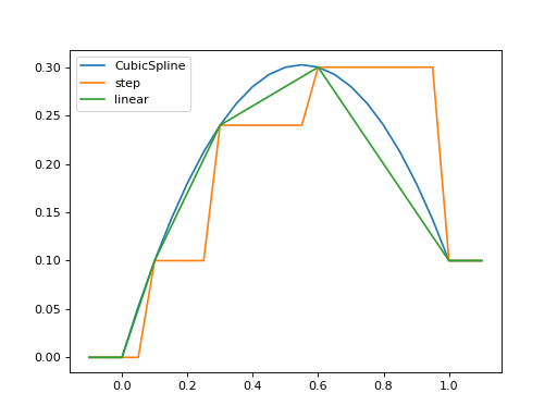
Per default, a cubic spline interpolation is used, but the order of the interpolation can be controlled with the order input: Outside the interpolation range, the first or last value are used.

times = np.array([0, 0.1, 0.3, 0.6, 1.0])
coeff = times * (1.1 - times)
tlist = np.linspace(-0.1, 1.1, 25)

H = QobjEvo([qeye(1), coeff], tlist=times)
plt.plot(tlist, [H(t).norm() for t in tlist], label="CubicSpline")

H = QobjEvo([qeye(1), coeff], tlist=times, order=0)
plt.plot(tlist, [H(t).norm() for t in tlist], label="step")

H = QobjEvo([qeye(1), coeff], tlist=times, order=1)
plt.plot(tlist, [H(t).norm() for t in tlist], label="linear")

plt.legend()

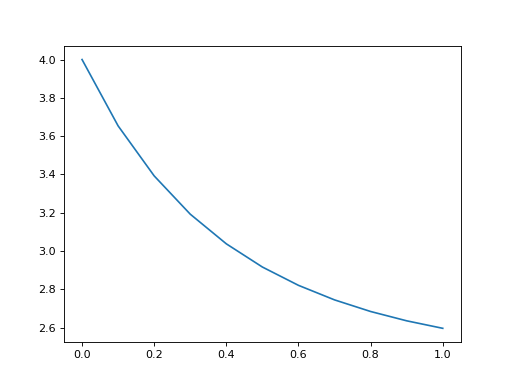
When using array coefficients in solver, if the time dependent quantum system is in list format, the solver tlist is used as times of the array. This is often not ideal as the interpolation is usually less precise close the extremities of the range. It is therefore better to create the QobjEvo using an extended range prior to the solver:

N = 5
times = np.linspace(-0.1, 1.1, 13)
coeff = np.exp(-times)

c_ops = [QobjEvo([destroy(N), coeff], tlist=times)]
tlist = np.linspace(0, 1, 11)
data = mesolve(qeye(N), basis(N, N-1), tlist, c_ops=c_ops, e_ops=[num(N)]).expect[0]
plt.plot(tlist, data)

Different coefficient types can be mixed in a QobjEvo.

Given the multiple choices of input style, the first question that arises is which option to choose? In short, the function based method (first option) is the most general, allowing for essentially arbitrary coefficients expressed via user defined functions. However, by automatically compiling your system into C++ code, the second option (string based) tends to be more efficient and run faster. Of course, for small system sizes and evolution times, the difference will be minor. Lastly the spline method is usually as fast the string method, but it cannot be modified once created.

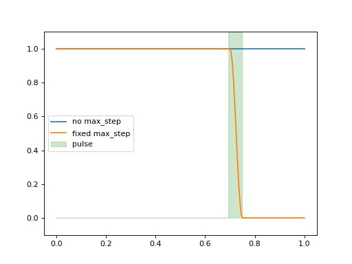
Working with pulses

Special care is needed when working with pulses. ODE solvers select the step length automatically and can miss thin pulses when not properly warned. Integrations methods with variable step sizes have the max_step option that control the maximum length of a single internal integration step. This value should be set to under half the pulse width to be certain they are not missed.

For example, the following pulse is missed without fixing the maximum step length.

def pulse(t):
    return 10 * np.pi * (0.7 < t < 0.75)

tlist = np.linspace(0, 1, 201)
H = [sigmaz(), [sigmax(), pulse]]
psi0 = basis(2,1)

data1 = sesolve(H, psi0, tlist, e_ops=num(2)).expect[0]
data2 = sesolve(H, psi0, tlist, e_ops=num(2), options={"max_step": 0.01}).expect[0]

plt.plot(tlist, data1, label="no max_step")
plt.plot(tlist, data2, label="fixed max_step")
plt.fill_between(tlist, [pulse(t) for t in tlist], color="g", alpha=0.2, label="pulse")
plt.ylim([-0.1, 1.1])
plt.legend(loc="center left")